Overview
What is BigBacter?
BigBacter is a Nextflow pipeline for routine bacterial genomic surveillance. It accepts raw reads or assemblies, clusters samples by genomic similarity, constructs core genome alignments, and produces phylogenetic trees and pairwise distance matrices - all in an iterative, database-backed workflow designed to grow with your dataset over time.
Key Features
🧬 Soft-core phylogenomics - retains substantially more phylogenetic signal than strict-core approaches by tolerating a configurable level of missing data
🧬 Automated reference selection - selects the most representative assembly per cluster using k-mer containment and assembly quality scoring; reuses the same reference on subsequent runs for consistent SNP distances
🧬 Dual distance metrics - reports both core-genome SNP distances and whole-genome containment scores to capture both SNP-level and accessory genome variation
Inputs
Read Processing
Reads can be supplied as FASTQ files (fastq_1 / fastq_2 columns) or downloaded automatically from NCBI using an SRA accession (sra column). Files exceeding the maximum read count set by max_reads (default: 2_000_000) will be randomly subsampled using seqtk. All reads are then quality filtered using fastp. If no reads are supplied, they will be derived from the genome assembly - read more here.
SNPs called from genome assemblies are considerably less reliable than those called from reads (Wick et al., 2025). Genome assemblers prioritize contiguity and completeness over base-level accuracy, meaning assembly errors can be indistinguishable from true variants. Unlike read-based variant calling, there is no per-site depth or quality information available to scrutinize the confidence of a call. Samples where reads are unavailable should be interpreted with caution, particularly in outbreak investigations where a small number of SNPs may be the basis for epidemiological conclusions.
Genome Assembly
Genome assemblies can be supplied as FASTA files (assembly column) or downloaded automatically from NCBI using a GenBank accession (genbank column). If no assembly is supplied, one will be created using shovill.
Taxonomy
Sample taxonomy is supplied via the taxa column. Samples are split into taxon-specific groups prior to cluster and core genome analysis. Species-level classification is appropriate for most cases - e.g., Escherichia coli.
If no taxonomy is provided, BigBacter will automatically assign species-level taxonomy using GAMBIT. GAMBIT uses k-mer based genome signatures to rapidly classify bacterial isolates. Automatically assigned taxonomy is subject to the limitations of GAMBIT’s reference database - for novel or poorly represented species, manual review of the assigned taxonomy is recommended before proceeding.
BigBacter does not perform extensive quality checks on genome assemblies or taxonomy assignments. It is strongly recommended that assemblies and taxonomy are generated and validated upstream using a dedicated workflow with robust QC - e.g., PHoeNIx, TheiaProk, or Bactopia.
Clustering
Samples are clustered within each taxonomic group using floc. Floc was developed at WA PHL for iterative sample clustering, accomplished using the sourmash containment method. This allows for a rough estimation of how much of the genome is shared between samples or between samples and existing clusters.
How Clustering Works
Each time BigBacter is run, newly assigned cluster information is saved to a database. The next time BigBacter is run for the same species, this database is automatically loaded so that new samples can be placed relative to all previously observed clusters. This iterative approach means that cluster assignments remain consistent over time.
Database Design
The floc database is intentionally simple compared to PopPUNK databases. Rather than storing cluster information in a single monolithic structure, floc saves data on a per-sample basis. This has several practical advantages:
- Individual samples can be removed from the database without rebuilding it from scratch (e.g., to exclude a contaminated or misidentified sample)
- Existing entries can be modified independently
- The database grows incrementally with each run, requiring no upfront preparation
A key consequence of this design is that BigBacter can be run with as little as a single sample for a given species. Databases are created on the fly during the first run and expanded with each subsequent run. This contrasts with PopPUNK, which requires a pre-built reference database to be created a priori before any samples can be assigned to clusters - a significant barrier when working with less common or emerging pathogens.
Miller et al. 2026 found that floc generally performs as well as or better than PopPUNK for cluster assignments, supporting the decision to adopt it as the clustering backbone for BigBacter v2.
Databases created using BigBacter v1 are not compatible with v2.
Visualizing Cluster Relationships
A neighbor-joining tree can be generated using the --clust_plot true parameter, allowing for investigation of overall cluster relationships across samples. Note that this tree is built from containment distances rather than sequence alignments, so the topology should not be interpreted as reflecting evolutionary history or directionality - branch lengths represent a non-directional magnitude of genomic divergence. See the example below:
Core Genome Analysis
Reference Selection
A reference genome is automatically selected for each cluster using bigbacter_select_ref.py. When a cluster contains multiple assemblies, the script evaluates each one and selects the candidate that best represents the full genomic diversity of the group.
The selection process works as follows:
- Contigs shorter than a minimum length (default:
300bp) are filtered out. - A MinHash sketch is built for each assembly using sourmash (default:
ksize=31,scaled=100). - A global sketch is created by merging all per-assembly sketches, representing the total k-mer diversity across all candidates.
-
Each assembly is scored using the formula:
score = containment × length / (n_contigs ^ penalty)Where
containmentmeasures what fraction of the global k-mer diversity is captured by the assembly,lengthrewards more complete assemblies, and the contigpenalty(default:0.2) discourages fragmented assemblies. The assembly with the highest score is selected as the reference. - The selected reference is written to
ref.fa.gzalong with a metadata file (ref.json) recording the sample name, genome length, and contig count.
The selected reference is saved to the BigBacter database for the cluster. On subsequent runs, if a reference already exists in the database for a given cluster, it is reused rather than re-selected. This ensures that all samples within a cluster are always mapped against the same reference, keeping SNP distances and alignments consistent over time. A new reference is only selected when a cluster is being processed for the first time.
Defining the Core Genome
Core genome analysis is performed using polycore. The process begins by mapping all samples in the cluster against the selected reference using Snippy, which generates per-sample alignments.
Rather than using a strict core - which requires data to be present in every sample at every site - BigBacter uses a soft core approach. As described by Taouk et al. (2025), strict cores can shrink dramatically as sample size and genome diversity increase, discarding potentially informative data. A soft core tolerates some missing data by applying a threshold: a site is included in the core genome if data are present in at least N% of samples (configurable; default targets the soft core). This preserves substantially more phylogenetic signal.
To assist the impact of adding each sample to the core genome analysis, polycore adds samples progressively by genome fraction size - larger, more complete assemblies are incorporated first. Samples that fall below the minimum genome size threshold are automatically excluded from core genome analysis, preventing low-quality assemblies from artificially eroding the core.
The per-sample SNP files generated by Snippy are saved to the BigBacter database on a per-sample basis. On subsequent runs, previously processed samples do not need to be re-mapped - their SNP files are retrieved directly from the database and combined with any newly mapped samples before the core genome is defined. This makes incremental runs substantially faster and means that adding new samples to an existing cluster only requires mapping the new samples rather than reprocessing the entire cluster from scratch.
Calling Variants
Variants are called by polycore directly from the soft-core genome alignment, producing a SNP alignment used for all downstream phylogenetic and distance analyses.
For clusters large enough to warrant recombination masking, a masked alignment is also generated using Gubbins. Gubbins identifies genomic regions consistent with horizontal gene transfer or recombination and masks them, so that inferred phylogenies and SNP distances reflect vertical inheritance rather than recombination noise.
Phylogenetic Analysis
Core SNP Tree
A maximum likelihood tree is inferred using IQ-TREE2 under the GTR+I+G model (general time reversible with a proportion of invariable sites and a discrete Gamma model for rate variation), with 1,000 rounds of rapid bootstrapping. While IQ-TREE2 supports automated model selection via ModelFinder, this can be prohibitively slow for routine surveillance. A standardized model was therefore selected based on published recommendations.
Ascertainment bias correction is applied via -fconst using the count of constant sites determined by polycore. This corrects for the fact that only variable sites are included in the SNP alignment, which would otherwise distort branch length estimates. Branch lengths are subsequently rescaled from substitutions per site to estimated nucleotide substitutions using the reference genome length.
To provide interpretable resolution across multiple scales of relatedness, trees are partitioned into sub-trees based on estimated pairwise nucleotide substitutions using DBSCAN (default threshold: 100 substitutions). This allows fine-scale outbreak investigation and broader population-level context to be viewed together.

Pairwise Distances
Two complementary distance metrics are calculated for each cluster.
Pairwise SNP distances are computed by polycore from the soft-core genome alignment. These provide a core-genome view of genomic similarity and are the primary metric for outbreak detection and cluster confirmation.
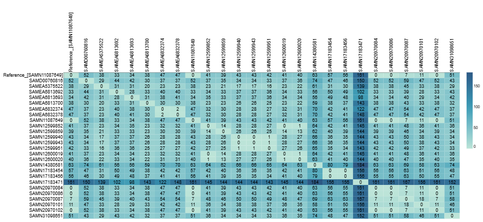
Pairwise percent average divergence is calculated from the average containment distance (floc) using the formula below:
This metric extends beyond the core genome to capture accessory genome differences - structural variation, gene gain/loss, and mobile elements that SNP-based methods miss entirely. The two metrics therefore complement each other and should be interpreted together.
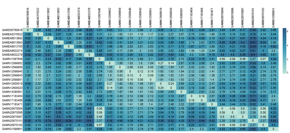
Containment distances are based on exact k-mer matches, which can cause them to both overestimate accessory differences in variable core regions and underestimate accessory differences in repetitive regions or paralogs. Interpret with caution!
Summary Report
Results are summarized at the taxon-cluster level in an interactive Microreact report. Each report includes:
- A maximum likelihood phylogenetic tree with bootstrap support
- Core and accessory genome pairwise distance matrices
- A genomic linkage summary for rapid identification of closely related samples
- A progressive core genome degradation plot illustrating how the soft-core genome shrinks as samples are added, which can be used to assess the impact of low-quality assemblies on the analysis
Want to see an example? 📄 Download this report, then upload it to microreact.org/upload to view it.
For a full description of report contents and how to interpret them, see the Outputs page.