# ------ Read in all tables and get counts ------ ##' @export#' match in wdrs or keep_na#' #' @description#' Find a match in WDRS or Keep_NA and assign it a new column. Used to get counts and filter#' #' @param df a dataframematch_in_wdrs_keep_na <-function(df){ df %>%mutate(in_wdrs =case_when( SEQUENCE_CLINICAL_ACCESSION %in%na.omit(wdrs_seq$SEQUENCE_CLINICAL_ACCESSION_NUMBER) | SEQUENCE_ACCESSION %in%na.omit(wdrs_seq$SEQUENCE_GISAID_STRAIN) ~1,TRUE~0 )) %>%mutate(in_keep_na =case_when( SEQUENCE_CLINICAL_ACCESSION %in%na.omit(keep_na2$SEQUENCE_CLINICAL_ACCESSION) | SEQUENCE_ACCESSION %in%na.omit(keep_na2$SEQUENCE_ACCESSION) ~1,TRUE~0 ))}# Read in keep_na - this reads in the saved keep_na pinkeep_na <-read_csv(file.path(here::here(),"docs/notebooks/data/keep_na.csv"))
New names:
• `` -> `...1`
Warning: One or more parsing issues, call `problems()` on your data frame for details,
e.g.:
  dat <- vroom(...)
  problems(dat)
Rows: 19855 Columns: 137
── Column specification ────────────────────────────────────────────────────────
Delimiter: ","
chr  (22): file_name, SEQUENCE_SPECIMEN, SEQUENCE_REASON, SEQUENCE_LAB, SEQU...
dbl   (3): ...1, CASE_ID, GISAID_ID_YEAR
lgl (112): SEQUENCE_SGTF, SEQUENCE_DATE, Virus name, Accession ID, Collectio...

ℹ Use `spec()` to retrieve the full column specification for this data.
ℹ Specify the column types or set `show_col_types = FALSE` to quiet this message.
# keep_na_extract() %>%# as_tibble() %>%# tweak_gisaid_id(.$SEQUENCE_ACCESSION) %>%# mutate(across(everything(), as.character))# Read in keep_na - this runs the keep_na read function to read in newest data# this will take ~ 10 min to run. Only necessary if the pin is out of date# keep_na <- keep_na_extract() %>%# as_tibble() %>%# tweak_gisaid_id(.$SEQUENCE_ACCESSION)# connectconnection <- DBI::dbConnect(odbc::odbc(), Driver = creds$default$conn_list_wdrs$Driver, Server = creds$default$conn_list_wdrs$Server, Database = creds$default$conn_list_wdrs$Database, Trusted_connection = creds$default$conn_list_wdrs$Trusted_connection, ApplicationIntent = creds$default$conn_list_wdrs$ApplicationIntent)wdrs_seq <- DBI::dbGetQuery( connection," SELECT * FROM DD_GCD_COVID19_SEQUENCING WHERE SEQUENCE_SPECIMEN = 'YES' AND CASE_STATUS IN (0, 3) ORDER BY SEQUENCE_ROSTER_PREPARE_DATE DESC; ")# Remove any recwdrs_seq <- wdrs_seq %>%mutate(in_keep_na =case_when( SEQUENCE_CLINICAL_ACCESSION_NUMBER %in%na.omit(keep_na$SEQUENCE_CLINICAL_ACCESSION) | SEQUENCE_GISAID_STRAIN %in%na.omit(keep_na$SEQUENCE_ACCESSION) ~1,TRUE~0 )) %>%as_tibble() %>%mutate(across(everything(), as.character)) %>%filter(SEQUENCE_ROSTER_PREPARE_DATE <'2023-09-11'|is.na(SEQUENCE_ROSTER_PREPARE_DATE))wdrs_count <- wdrs_seq %>%# filter(in_keep_na == 0) %>%nrow()# This keep_na count needs to run below WDRS chunk because it needs to remove# any records that are in WDRSkeep_na2 <- keep_na %>%mutate(in_wdrs =if_else( SEQUENCE_CLINICAL_ACCESSION %in%na.omit( wdrs_seq$SEQUENCE_CLINICAL_ACCESSION_NUMBER ),1,0 ) ) %>%mutate(in_wdrs_SA =if_else( SEQUENCE_ACCESSION %in%na.omit( wdrs_seq$SEQUENCE_GISAID_STRAIN ),1,0 ) ) %>% dplyr::filter(in_wdrs ==0& in_wdrs_SA ==0)keep_na_count <-nrow(keep_na2)# Read in for_reviewfor_review_df <-for_review_extract() %>%# Find a match in WDRS or keep_namatch_in_wdrs_keep_na() %>%# Split SEQUENCE_ACCESSION for partial matchingtweak_gisaid_id(.$SEQUENCE_ACCESSION)for_review_count <- for_review_df %>%filter(in_wdrs ==0& in_keep_na ==0) %>%nrow()# Read in fuzzyfuzzy_df <-fuzzy_extract() %>%# Find a match in WDRS or keep_namatch_in_wdrs_keep_na() %>%# Split SEQUENCE_ACCESSION for partial matchingtweak_gisaid_id(.$SEQUENCE_ACCESSION)fuzzy_count <- fuzzy_df %>%filter(in_wdrs ==0& in_keep_na ==0) %>%nrow()
Count Summary
In [3]:
In [4]:
# ------ Create Final Table of Counts ------ ## Get the Countspipeline_counts <-tribble(~Location, ~Count,"For Review", for_review_count,"Fuzzy Review", fuzzy_count,"Keep NA", keep_na_count,"WDRS", wdrs_count) %>%# Get the Percentsmutate(freq = scales::label_percent()(Count /sum(Count))) %>%# Get the Totals janitor::adorn_totals()# Take the counts and put them in a table.# use the gt table for html stuff# Convert to a GT table and style it(gt_counts <- pipeline_counts %>%gt() %>%cols_merge_n_pct(col_n = Count,col_pct = freq ) %>%fmt_number(columns = Count,decimals =0,use_seps = T ) %>%# Highlight the WDRS rowgt_highlight_rows(rows = Location =="WDRS",fill ="#8b7d7b",bold_target_only =TRUE,target_col = Count ) %>%cols_align("left") %>%tab_header(title =md("Covid Sequencing Pipeline Counts")) %>%style_table())# make a kable table - these are the only tables that can be output with a manuscript project# pipeline_counts %>% # mutate(Count = paste0(Count," (",freq,")")) %>% # select(-freq) %>%# knitr::kable()
Count of sequences matching to WDRS cases
Covid Sequencing Pipeline Counts
Location
Count
For Review
220 (0.13%)
Fuzzy Review
569 (0.33%)
Keep NA
5,710 (3.32%)
WDRS
165,551 (96.22%)
Total
172,050 (-)
Counts by Lab
In [5]:
In [6]:
# ------ Summary of the Tables ------ #lab_counts <- wdrs_seq %>%mutate(SEQUENCE_LAB = forcats::fct_explicit_na(SEQUENCE_LAB)) %>%mutate(SEQUENCE_STATUS = forcats::fct_explicit_na(SEQUENCE_STATUS)) %>%select(SEQUENCE_STATUS,SEQUENCE_LAB) %>%count(SEQUENCE_STATUS,SEQUENCE_LAB) %>%pivot_wider(names_from = SEQUENCE_STATUS,values_from = n) %>%arrange(desc(Complete)) %>% janitor::adorn_totals()# Get counts by lab by status gt(gt_lab_counts <- lab_counts %>%gt() %>%fmt(columns =-SEQUENCE_LAB,fns =function(x) ifelse(is.na(x), "—", x) ) %>%data_color(columns = Complete,rows = SEQUENCE_LAB !="Total",direction ="column", palette ="Purples",alpha =1) %>%style_table())# Get counts by status kable# options(knitr.kable.NA = '-')# lab_counts %>%# knitr::kable()
Count of sequences by lab and status
SEQUENCE_LAB
Complete
Failed
Low Quality
Not Done
(Missing)
UW Virology
67642
1507
648
—
2
PHL
29497
2497
850
1
—
Labcorp
19029
7530
37
—
1
NW Genomics
15851
523
2158
—
—
Quest
3923
—
198
—
—
Altius
3523
140
33
—
—
Fulgent Genetics
2859
—
—
—
—
PHL/Bedford
2857
—
—
—
—
SCAN/Bedford
996
1
7
—
—
Aegis
934
4
5
—
—
Curative Labs
623
—
26
—
—
KP WA Research Inst
281
—
—
—
—
USAFSAM
275
—
—
—
—
CDC
207
3
1
—
—
Providence Swedish
173
—
—
—
—
Helix
143
8
—
—
—
Lauring Lab
118
—
—
—
—
Atlas Genomics
68
—
21
—
—
Boise VA
64
3
—
—
—
OHSU
61
—
—
—
—
SFS/Bedford
48
—
5
—
—
IDBOL
40
—
—
—
—
Gravity Diagnostics
36
—
—
—
—
ASU
33
—
—
—
—
OSPHL
14
1
—
—
—
USAMRIID
9
—
—
—
—
Infinity Biologix
7
—
—
—
—
Grubaugh Lab
2
—
—
—
—
Montana Public Health Lab
2
—
—
—
—
Flow Diagnostics
1
—
—
—
—
Grittman Medical Center
1
—
—
—
—
Naval Health Research Center
1
—
—
—
—
NW GENOMICS
1
—
—
—
—
Providence_Swedish
1
—
—
—
—
SCAB/Bedford
1
—
—
—
—
SFS/ Bedford
1
—
—
—
—
The Jackson Laboratory
1
—
—
—
—
(Missing)
1
1
—
—
16
Total
149324
12218
3989
1
19
Counts by lab
These are counts before we switched over to the 2.0 pipeline
In [7]:
In [8]:
(count_by_lab <- wdrs_seq %>%count(SEQUENCE_LAB) %>%arrange(desc(n)) %>%summarize( n,x_scaled = n /nrow(wdrs_seq) *100,.by = SEQUENCE_LAB ) %>%gt() %>%gt_plt_bar_pct(column = x_scaled,scaled =TRUE,labels =TRUE,font_size ="12px",fill ="#8b7d7b" ) %>%tab_header(title =md("Number of Sequences by Lab"),subtitle =md("Before 2023-06-01 switch to 2.0 pipeline")) %>%fmt_number(columns = n,decimals =0,use_seps = T ) %>%cols_label(SEQUENCE_LAB ='Sequencing Lab',n ='Count',x_scaled ='Percent of Total Sequences' ) %>%style_table())
Count of sequences by lab and status during the sequencing pipeline 1.0 phase
Number of Sequences by Lab
Before 2023-06-01 switch to 2.0 pipeline
Sequencing Lab
Count
Percent of Total Sequences
UW Virology
69,799
42.2%
PHL
32,845
19.8%
Labcorp
26,597
16.1%
NW Genomics
18,532
11.2%
Quest
4,121
2.5%
Altius
3,696
2.2%
Fulgent Genetics
2,859
1.7%
PHL/Bedford
2,857
1.7%
SCAN/Bedford
1,004
0.6%
Aegis
943
0.6%
Curative Labs
649
0.4%
KP WA Research Inst
281
0.2%
USAFSAM
275
0.2%
CDC
211
0.1%
Providence Swedish
173
0.1%
Helix
151
0.1%
Lauring Lab
118
0.1%
Atlas Genomics
89
0.1%
Boise VA
67
0%
OHSU
61
0%
SFS/Bedford
53
0%
IDBOL
40
0%
Gravity Diagnostics
36
0%
ASU
33
0%
NA
18
0%
OSPHL
15
0%
USAMRIID
9
0%
Infinity Biologix
7
0%
Grubaugh Lab
2
0%
Montana Public Health Lab
2
0%
Flow Diagnostics
1
0%
Grittman Medical Center
1
0%
NW GENOMICS
1
0%
Naval Health Research Center
1
0%
Providence_Swedish
1
0%
SCAB/Bedford
1
0%
SFS/ Bedford
1
0%
The Jackson Laboratory
1
0%
Create stacked bar plots
created by Philip Crain
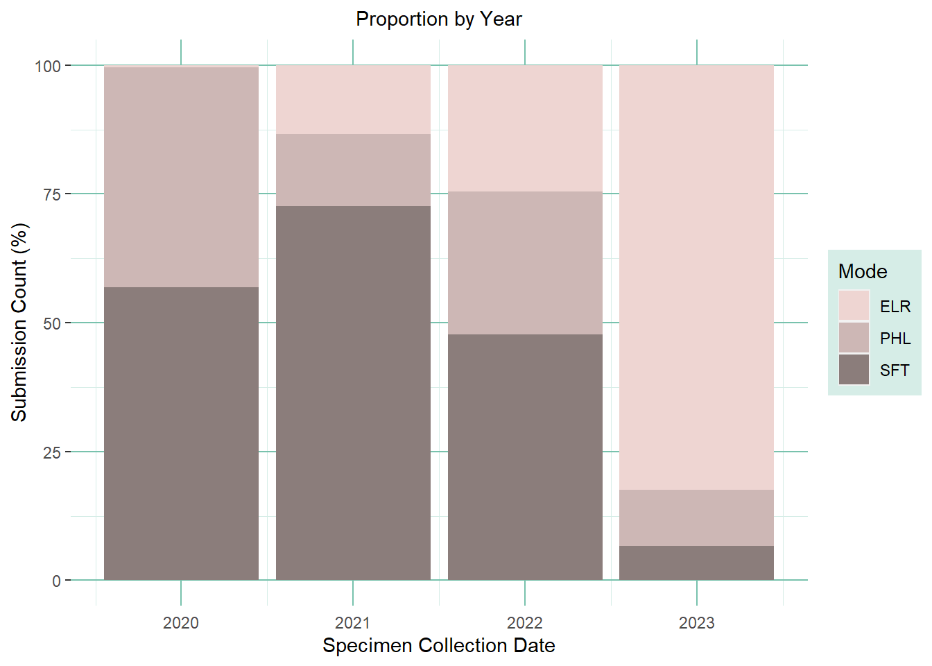
Proportion Plot
make a plot based on the proportion stratified by mode
note: a few labs switched from Template to ELR and they were not always hard cut offs. Need to combine data with the entire table in order to identify which records are template and which are coming from ELR.
In [9]:
WDRS_Entire <-dbGetQuery(connection, " SELECT DISTINCT CASE_ID, FILLER__ORDER__NUM, SPECIMEN__COLLECTION__DTTM, SUBMITTER, PATIENT__CENTRIC__OBSERVATION, PATIENT__CENTRIC__OBSERVATION__VALUE, TEST__RESULT, TEST__RESULT__NOTE, TEST__REQUEST__NOTE FROM [dbo].[DD_ELR_DD_ENTIRE] WHERE WDRS__TEST__PERFORMED = 'SARS CoV-2 Sequencing'")wdrs_seq_prep <- wdrs_seq %>%filter(SEQUENCE_ROSTER_PREPARE_DATE <'2023-09-11'|is.na(SEQUENCE_ROSTER_PREPARE_DATE)) %>%mutate(sc_year = lubridate::year(CASE_CREATE_DATE),in_elr =if_else(CASE_ID %in% WDRS_Entire$CASE_ID,1,0),submission_route =factor(case_when(# str_detect(toupper(SEQUENCE_LAB),"AEGIS|HELIX|QUEST|LABCORP") ~ "ELR",# some labs have submitted template and ELR, so need a better way of finding them# use the ELR table to determine which are ELR in_elr ==1~"ELR", in_elr ==0&str_detect(toupper(SEQUENCE_LAB),"PHL") ~"PHL",TRUE~"SFT" ) ) )
In [10]:
library(ggplot2)
Warning: package 'ggplot2' was built under R version 4.2.2
(prop_plot <- wdrs_seq_prep %>% ggplot2::ggplot(aes(x=sc_year,fill=submission_route)) +geom_bar(position="fill") +# scale_x_date() +scale_y_continuous(labels =~.x*100) +scale_fill_manual(values=c("mistyrose2", "mistyrose3", "mistyrose4")) +labs(title='Proportion by Year',fill='Mode') +xlab('Specimen Collection Date') +ylab('Submission Count (%)') +theme(plot.title =element_text(hjust =0.5, size=rel(1)),axis.ticks.x =element_line(color =NA),panel.background =element_rect(fill ='transparent'),plot.background =element_rect(fill ='transparent', color =NA),panel.grid.major.y =element_line(color ='#78c2ad'),panel.grid.major.x =element_line(color ='#78c2ad'),panel.grid.minor.y =element_line(color ='#d6ede7'),panel.grid.minor.x =element_line(color ='#d6ede7'),legend.background =element_rect(fill ='#d6ede7'),#legend.key = element_rect(fill = 'transparent'),# legend.position = "none" #remove legend to save space when next to the yearly version png ) )
Count Plot
In [11]:
### Create yearly count stacked bar: --------------------------------(count_plot <- wdrs_seq_prep %>%ggplot(aes(x=sc_year, fill=submission_route)) +geom_bar(position='stack') +# scale_x_date() +scale_y_continuous(labels = scales::label_comma()) +scale_fill_manual(values=c("mistyrose2", "mistyrose3", "mistyrose4")) +labs(title='Count by Year',fill='Mode') +xlab('Specimen Collection Date') +ylab('Submission Count (n)') +theme(plot.title =element_text(hjust =0.5, size=rel(1)),axis.ticks.x =element_line(color =NA),panel.background =element_rect(fill ='transparent'),plot.background =element_rect(fill ='transparent', color =NA),panel.grid.major.y =element_line(color ='#78c2ad'),panel.grid.major.x =element_line(color ='#78c2ad'),panel.grid.minor.y =element_line(color ='#d6ede7'),panel.grid.minor.x =element_line(color ='#d6ede7'),legend.background =element_rect(fill ='#d6ede7'),# legend.key = element_rect(fill = 'transparent'),#legend.position = "none" #remove legend to save space when next to the yearly version png ) )
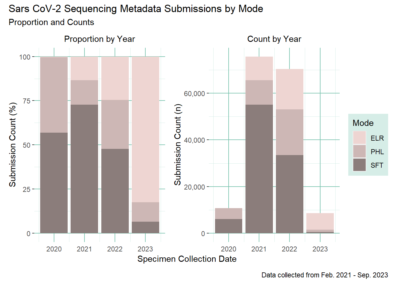
Combine the plots
Use patchwork to combine the plots
In [12]:
library(patchwork)(prop_plot + count_plot) +plot_layout(guides="collect", axes ="collect_x") +plot_annotation(title ='Sars CoV-2 Sequencing Metadata Submissions by Mode',subtitle ='Proportion and Counts',caption ='Data collected from Feb. 2021 - Sep. 2023' )
Count and proportion of sequencing metadata submissions by mode